Artificial information filtering

In simple terms the bitinformation is retrieved by checking how variable a bit pattern is. However, this approach cannot distinguish between actual information content and artifical information content. By studying the distribution of the information content the user can often identify clear cut-offs of real information content and artificial information content.

The following example shows how such a separation of real information and artificial information can look like. To do so, artificial information is artificially added to an example dataset by applying linear quantization. Linear quantization is often applied to climate datasets (e.g. ERA5) and needs to be accounted for in order to retrieve meaningful bitinformation content. An algorithm that aims at detecting this artificial information itself is introduced.

import xarray as xr
import xbitinfo as xb
import numpy as np

/home/docs/checkouts/readthedocs.org/user_builds/xbitinfo/conda/latest/lib/python3.12/site-packages/tqdm/auto.py:21: TqdmWarning: IProgress not found. Please update jupyter and ipywidgets. See https://ipywidgets.readthedocs.io/en/stable/user_install.html
  from .autonotebook import tqdm as notebook_tqdm

Loading example dataset

We use here the openly accessible CONUS dataset. The dataset is available at full precision.

ds = xr.open_zarr(
    "s3://hytest/conus404/conus404_monthly.zarr",
    storage_options={
        "anon": True,
        "requester_pays": False,
        "client_kwargs": {"endpoint_url": "https://usgs.osn.mghpcc.org"},
    },
)
# selecting water vapor mixing ratio at 2 meters
data = ds["ACSWDNT"]
# select subset of data for demonstration purposes
chunk = data.isel(time=slice(0, 2), y=slice(0, 1015), x=slice(0, 1050))
chunk

<xarray.DataArray 'ACSWDNT' (time: 2, y: 1015, x: 1050)> Size: 9MB
dask.array<getitem, shape=(2, 1015, 1050), dtype=float32, chunksize=(2, 350, 350), chunktype=numpy.ndarray>
Coordinates:
    lat      (y, x) float32 4MB dask.array<chunksize=(350, 350), meta=np.ndarray>
    lon      (y, x) float32 4MB dask.array<chunksize=(350, 350), meta=np.ndarray>
  * time     (time) datetime64[ns] 16B 1979-10-31 1979-11-30
  * x        (x) float64 8kB -2.732e+06 -2.728e+06 ... 1.46e+06 1.464e+06
  * y        (y) float64 8kB -2.028e+06 -2.024e+06 ... 2.024e+06 2.028e+06
Attributes:
    description:         ACCUMULATED DOWNWELLING SHORTWAVE FLUX AT TOP
    grid_mapping:        crs
    integration_length:  month accumulation
    long_name:           Accumulated downwelling shortwave radiation flux at top
    units:               J m-2

xarray.DataArray

'ACSWDNT'

• time: 2
• y: 1015
• x: 1050

• dask.array<chunksize=(2, 350, 350), meta=np.ndarray>

  Array Chunk Bytes 8.13 MiB 0.93 MiB Shape (2, 1015, 1050) (2, 350, 350) Dask graph 9 chunks in 3 graph layers Data type float32 numpy.ndarray

• Coordinates: (5)
  • lat
    (y, x)
    float32
    dask.array<chunksize=(350, 350), meta=np.ndarray>

    description :

    LATITUDE, SOUTH IS NEGATIVE

    grid_mapping :

    crs

    long_name :

    Latitude, south is negative

    units :

    degree_north

    Array Chunk Bytes 4.07 MiB 478.52 kiB Shape (1015, 1050) (350, 350) Dask graph 9 chunks in 3 graph layers Data type float32 numpy.ndarray

  • lon
    (y, x)
    float32
    dask.array<chunksize=(350, 350), meta=np.ndarray>

    description :

    LONGITUDE, WEST IS NEGATIVE

    grid_mapping :

    crs

    long_name :

    Longitude, west is negative

    units :

    degree_east

    Array Chunk Bytes 4.07 MiB 478.52 kiB Shape (1015, 1050) (350, 350) Dask graph 9 chunks in 3 graph layers Data type float32 numpy.ndarray

  • time
    (time)
    datetime64[ns]
    1979-10-31 1979-11-30

    array(['1979-10-31T00:00:00.000000000', '1979-11-30T00:00:00.000000000'],
          dtype='datetime64[ns]')

  • x
    (x)
    float64
    -2.732e+06 -2.728e+06 ... 1.464e+06

    long_name :

    x coordinate of projection

    standard_name :

    projection_x_coordinate

    units :

    m

    array([-2732000., -2728000., -2724000., ...,  1456000.,  1460000.,  1464000.])

  • y
    (y)
    float64
    -2.028e+06 -2.024e+06 ... 2.028e+06

    long_name :

    y coordinate of projection

    standard_name :

    projection_y_coordinate

    units :

    m

    array([-2028000., -2024000., -2020000., ...,  2020000.,  2024000.,  2028000.])

• Indexes: (3)
  • time
    PandasIndex

    PandasIndex(DatetimeIndex(['1979-10-31', '1979-11-30'], dtype='datetime64[ns]', name='time', freq=None))

  • x
    PandasIndex

    PandasIndex(Index([-2732000.0, -2728000.0, -2724000.0, -2720000.0, -2716000.0, -2712000.0,
           -2708000.0, -2704000.0, -2700000.0, -2696000.0,
           ...
            1428000.0,  1432000.0,  1436000.0,  1440000.0,  1444000.0,  1448000.0,
            1452000.0,  1456000.0,  1460000.0,  1464000.0],
          dtype='float64', name='x', length=1050))

  • y
    PandasIndex

    PandasIndex(Index([-2027999.9999999958, -2023999.9999999958, -2019999.9999999958,
           -2015999.9999999958, -2011999.9999999958, -2007999.9999999958,
           -2003999.9999999958, -1999999.9999999958, -1995999.9999999958,
           -1991999.9999999958,
           ...
            1992000.0000000042,  1996000.0000000042,  2000000.0000000042,
            2004000.0000000042,  2008000.0000000042,  2012000.0000000042,
            2016000.0000000042,  2020000.0000000042,  2024000.0000000042,
            2028000.0000000042],
          dtype='float64', name='y', length=1015))

• Attributes: (5)

  description :

  ACCUMULATED DOWNWELLING SHORTWAVE FLUX AT TOP

  grid_mapping :

  crs

  integration_length :

  month accumulation

  long_name :

  Accumulated downwelling shortwave radiation flux at top

  units :

  J m-2

Creating dataset copy with artificial information

Functions to encode and decode

Artificial information filtering

In simple terms the bitinformation is retrieved by checking how variable a bit pattern is. However, this approach cannot distinguish between actual information content and artifical information content. By studying the distribution of the information content the user can often identify clear cut-offs of real information content and artificial information content.

The following example shows how such a separation of real information and artificial information can look like. To do so, artificial information is artificially added to an example dataset by applying linear quantization. Linear quantization is often applied to climate datasets (e.g. ERA5) and needs to be accounted for in order to retrieve meaningful bitinformation content. An algorithm that aims at detecting this artificial information itself is introduced.

import xarray as xr
import xbitinfo as xb
import numpy as np

Loading example dataset

We use here the openly accessible CONUS dataset. The dataset is available at full precision.

ds = xr.open_zarr(
    "s3://hytest/conus404/conus404_monthly.zarr",
    storage_options={
        "anon": True,
        "requester_pays": False,
        "client_kwargs": {"endpoint_url": "https://usgs.osn.mghpcc.org"},
    },
)
# selecting water vapor mixing ratio at 2 meters
data = ds["ACSWDNT"]
# select subset of data for demonstration purposes
chunk = data.isel(time=slice(0, 2), y=slice(0, 1015), x=slice(0, 1050))
chunk

<xarray.DataArray 'ACSWDNT' (time: 2, y: 1015, x: 1050)> Size: 9MB
dask.array<getitem, shape=(2, 1015, 1050), dtype=float32, chunksize=(2, 350, 350), chunktype=numpy.ndarray>
Coordinates:
    lat      (y, x) float32 4MB dask.array<chunksize=(350, 350), meta=np.ndarray>
    lon      (y, x) float32 4MB dask.array<chunksize=(350, 350), meta=np.ndarray>
  * time     (time) datetime64[ns] 16B 1979-10-31 1979-11-30
  * x        (x) float64 8kB -2.732e+06 -2.728e+06 ... 1.46e+06 1.464e+06
  * y        (y) float64 8kB -2.028e+06 -2.024e+06 ... 2.024e+06 2.028e+06
Attributes:
    description:         ACCUMULATED DOWNWELLING SHORTWAVE FLUX AT TOP
    grid_mapping:        crs
    integration_length:  month accumulation
    long_name:           Accumulated downwelling shortwave radiation flux at top
    units:               J m-2

xarray.DataArray

'ACSWDNT'

• time: 2
• y: 1015
• x: 1050

• dask.array<chunksize=(2, 350, 350), meta=np.ndarray>

  Array Chunk Bytes 8.13 MiB 0.93 MiB Shape (2, 1015, 1050) (2, 350, 350) Dask graph 9 chunks in 3 graph layers Data type float32 numpy.ndarray

• Coordinates: (5)
  • lat
    (y, x)
    float32
    dask.array<chunksize=(350, 350), meta=np.ndarray>

    description :

    LATITUDE, SOUTH IS NEGATIVE

    grid_mapping :

    crs

    long_name :

    Latitude, south is negative

    units :

    degree_north

    Array Chunk Bytes 4.07 MiB 478.52 kiB Shape (1015, 1050) (350, 350) Dask graph 9 chunks in 3 graph layers Data type float32 numpy.ndarray

  • lon
    (y, x)
    float32
    dask.array<chunksize=(350, 350), meta=np.ndarray>

    description :

    LONGITUDE, WEST IS NEGATIVE

    grid_mapping :

    crs

    long_name :

    Longitude, west is negative

    units :

    degree_east

    Array Chunk Bytes 4.07 MiB 478.52 kiB Shape (1015, 1050) (350, 350) Dask graph 9 chunks in 3 graph layers Data type float32 numpy.ndarray

  • time
    (time)
    datetime64[ns]
    1979-10-31 1979-11-30

    array(['1979-10-31T00:00:00.000000000', '1979-11-30T00:00:00.000000000'],
          dtype='datetime64[ns]')

  • x
    (x)
    float64
    -2.732e+06 -2.728e+06 ... 1.464e+06

    long_name :

    x coordinate of projection

    standard_name :

    projection_x_coordinate

    units :

    m

    array([-2732000., -2728000., -2724000., ...,  1456000.,  1460000.,  1464000.])

  • y
    (y)
    float64
    -2.028e+06 -2.024e+06 ... 2.028e+06

    long_name :

    y coordinate of projection

    standard_name :

    projection_y_coordinate

    units :

    m

    array([-2028000., -2024000., -2020000., ...,  2020000.,  2024000.,  2028000.])

• Indexes: (3)
  • time
    PandasIndex

    PandasIndex(DatetimeIndex(['1979-10-31', '1979-11-30'], dtype='datetime64[ns]', name='time', freq=None))

  • x
    PandasIndex

    PandasIndex(Index([-2732000.0, -2728000.0, -2724000.0, -2720000.0, -2716000.0, -2712000.0,
           -2708000.0, -2704000.0, -2700000.0, -2696000.0,
           ...
            1428000.0,  1432000.0,  1436000.0,  1440000.0,  1444000.0,  1448000.0,
            1452000.0,  1456000.0,  1460000.0,  1464000.0],
          dtype='float64', name='x', length=1050))

  • y
    PandasIndex

    PandasIndex(Index([-2027999.9999999958, -2023999.9999999958, -2019999.9999999958,
           -2015999.9999999958, -2011999.9999999958, -2007999.9999999958,
           -2003999.9999999958, -1999999.9999999958, -1995999.9999999958,
           -1991999.9999999958,
           ...
            1992000.0000000042,  1996000.0000000042,  2000000.0000000042,
            2004000.0000000042,  2008000.0000000042,  2012000.0000000042,
            2016000.0000000042,  2020000.0000000042,  2024000.0000000042,
            2028000.0000000042],
          dtype='float64', name='y', length=1015))

• Attributes: (5)

  description :

  ACCUMULATED DOWNWELLING SHORTWAVE FLUX AT TOP

  grid_mapping :

  crs

  integration_length :

  month accumulation

  long_name :

  Accumulated downwelling shortwave radiation flux at top

  units :

  J m-2

Creating dataset copy with artificial information

Functions to encode and decode

# Encoding function to compress data
def encode(chunk, scale, offset, dtype, astype):
    enc = (chunk - offset) * scale
    enc = np.around(enc)
    enc = enc.astype(astype, copy=False)
    return enc


# Decoding function to decompress data
def decode(enc, scale, offset, dtype, astype):
    dec = (enc / scale) + offset
    dec = dec.astype(dtype, copy=False)
    return dec

Transform dataset to introduce artificial information

xmin = np.min(chunk)
xmax = np.max(chunk)
scale = (2**16 - 1) / (xmax - xmin)
offset = xmin
enc = encode(chunk, scale, offset, "f4", "u2")
dec = decode(enc, scale, offset, "f4", "u2")

Comparison of bitinformation

# original dataset without artificial information
orig_info = xb.get_bitinformation(
    xr.Dataset({"w/o artif. info": chunk}),
    dim="x",
    implementation="python",
)

# dataset with artificial information
arti_info = xb.get_bitinformation(
    xr.Dataset({"w artif. info": dec}),
    dim="x",
    implementation="python",
)

# plotting distribution of bitwise information content
info = xr.merge([orig_info, arti_info])
plot = xb.plot_bitinformation(info)

  0%|          | 0/1 [00:00<?, ?it/s]

Processing var: w/o artif. info for dim: x:   0%|          | 0/1 [00:00<?, ?it/s]

Processing var: w/o artif. info for dim: x: 100%|██████████| 1/1 [00:05<00:00,  5.64s/it]

Processing var: w/o artif. info for dim: x: 100%|██████████| 1/1 [00:05<00:00,  5.64s/it]

  0%|          | 0/1 [00:00<?, ?it/s]

Processing var: w artif. info for dim: x:   0%|          | 0/1 [00:00<?, ?it/s]

Processing var: w artif. info for dim: x: 100%|██████████| 1/1 [00:05<00:00,  5.56s/it]

Processing var: w artif. info for dim: x: 100%|██████████| 1/1 [00:05<00:00,  5.56s/it]

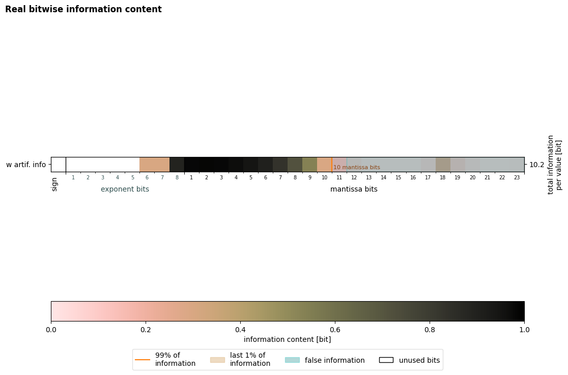
The figure reveals that artificial information is introduced by applying linear quantization.

keepbits = xb.get_keepbits(info, inflevel=[0.99])
print(
    f"The number of keepbits increased from {keepbits['w/o artif. info'].item(0)} bits in the original dataset to {keepbits['w artif. info'].item(0)} bits in the dataset with artificial information."
)

The number of keepbits increased from 10 bits in the original dataset to 18 bits in the dataset with artificial information.

In the following, a gradient based filter is introduced to remove this artificial information again so that even in case artificial information is present in a dataset the number of keepbits remains similar.

Artificial information filter

The filter gradient works as follows:

1. It determines the Cumulative Distribution Function(CDF) of the bitwise information content

2. It computes the gradient of the CDF to identify points where the gradient becomes close to a given tolerance indicating a drop in information.

3. Simultaneously, it keeps track of the minimum cumulative sum of information content which is threshold here, which signifies at least this much fraction of total information needs to be passed.

4. So the bit where the intersection of the gradient reaching the tolerance and the cumulative sum exceeding the threshold is our TrueKeepbits. All bits beyond this index are assumed to contain artificial information and are set to zero in order to cut them off.

5. You can see the above concept implemented in the function get_cdf_without_artificial_information in xbitinfo.py

Please note that this filter relies on a clear separation between real and artificial information content and might not work in all cases.

xb.get_keepbits(
    arti_info,
    inflevel=[0.99],
    information_filter="Gradient",
    **{"threshold": 0.7, "tolerance": 0.001}
)

<xarray.Dataset> Size: 20B
Dimensions:        (inflevel: 1)
Coordinates:
    dim            <U1 4B 'x'
  * inflevel       (inflevel) float64 8B 0.99
Data variables:
    w artif. info  (inflevel) int64 8B 10

xarray.Dataset

• Dimensions:
  • inflevel: 1
• Coordinates: (2)
  • dim
    ()
    <U1
    'x'

    description :

    dimension of the source dataset along which the bitwise information has been analysed.

    array('x', dtype='<U1')

  • inflevel
    (inflevel)
    float64
    0.99

    array([0.99])

• Data variables: (1)
  • w artif. info
    (inflevel)
    int64
    10

    array([10])

• Indexes: (1)
  • inflevel
    PandasIndex

    PandasIndex(Index([0.99], dtype='float64', name='inflevel'))

• Attributes: (0)

With the application of the filter the keepbits are closer/identical to their original value in the dataset without artificial information. The plot of the bitinformation visualizes this:

plot = xb.plot_bitinformation(arti_info, information_filter="Gradient")